Climate Sensitivity
Climate sensitivity comes in several flavors, with a correspondence between complexity and relevance. We review these various notions of climate sensitivity, as well as their interconnectedness and specific properties, in Jeevanjee et al. (2025).
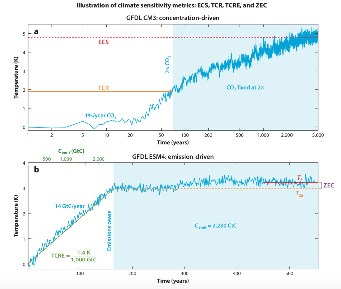
Figure left: Illustration of different climate sensitivity metrics using a physical climate model (GFDL-CM3) and an Earth system model with an interactive carbon cycle (GFDL-ESM4). Top: The Equilibrium Climate Sensitivity (ECS) of GFDL-CM3 is the long-term temperature response to a doubling of CO2 concentrations, while the Transient Climate Response (TCR) is the temperature when CO2 concentrations first reach a doubling after increasing at 1%/year. Bottom: The Transient Climate Response to cumulative Emissions (TCRE) of GFDL-ESM4 is the slope of transient temperature change vs cumulative CO2 emissions (green axis), while the Zero Emissions Commitment is the temperature change between emissions cessation and long-term equilibrium.
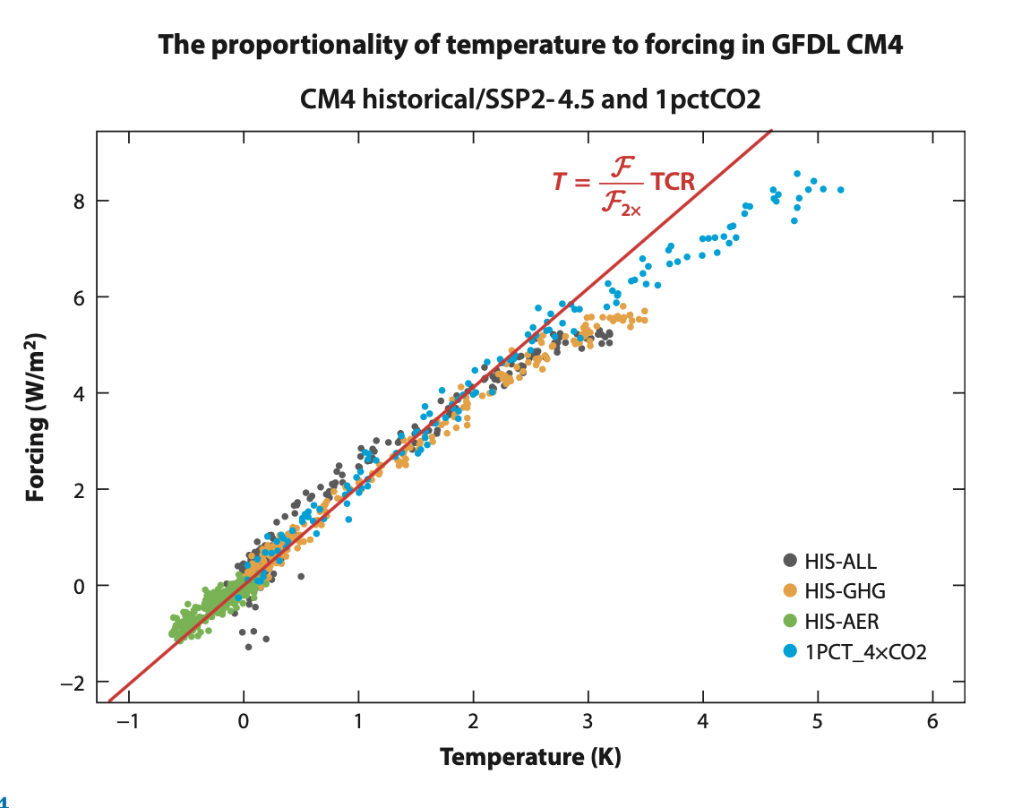
In particular, the Transient Climate Response (TCR) is relevant for a large class of transient climate change scenarios. The figure to the right shows that when the radiative forcing is plotted against temperature for transient climate change simulations, the relationship is largely linear and is mostly captured by simply scaling the TCR.
Figure right: Scatterplot of annual mean, global mean forcing vs temperature for a variety of climate change scenarios simulated with GFDL-CM4. The "HIS" simulations are historical extended out to 2100 using the SSP2-4.5 scenario, where "HIS-ALL" includes all forcing agents, "HIS-GHG" includes only greenhouse gases, and "HIS-AER" includes only aerosol forcing. The "1PCT_4XCO2" simulation has CO2 increasing at 1%/yr until CO2 quadruples.
Anvil Cloud Fraction and Convective Mass Flux
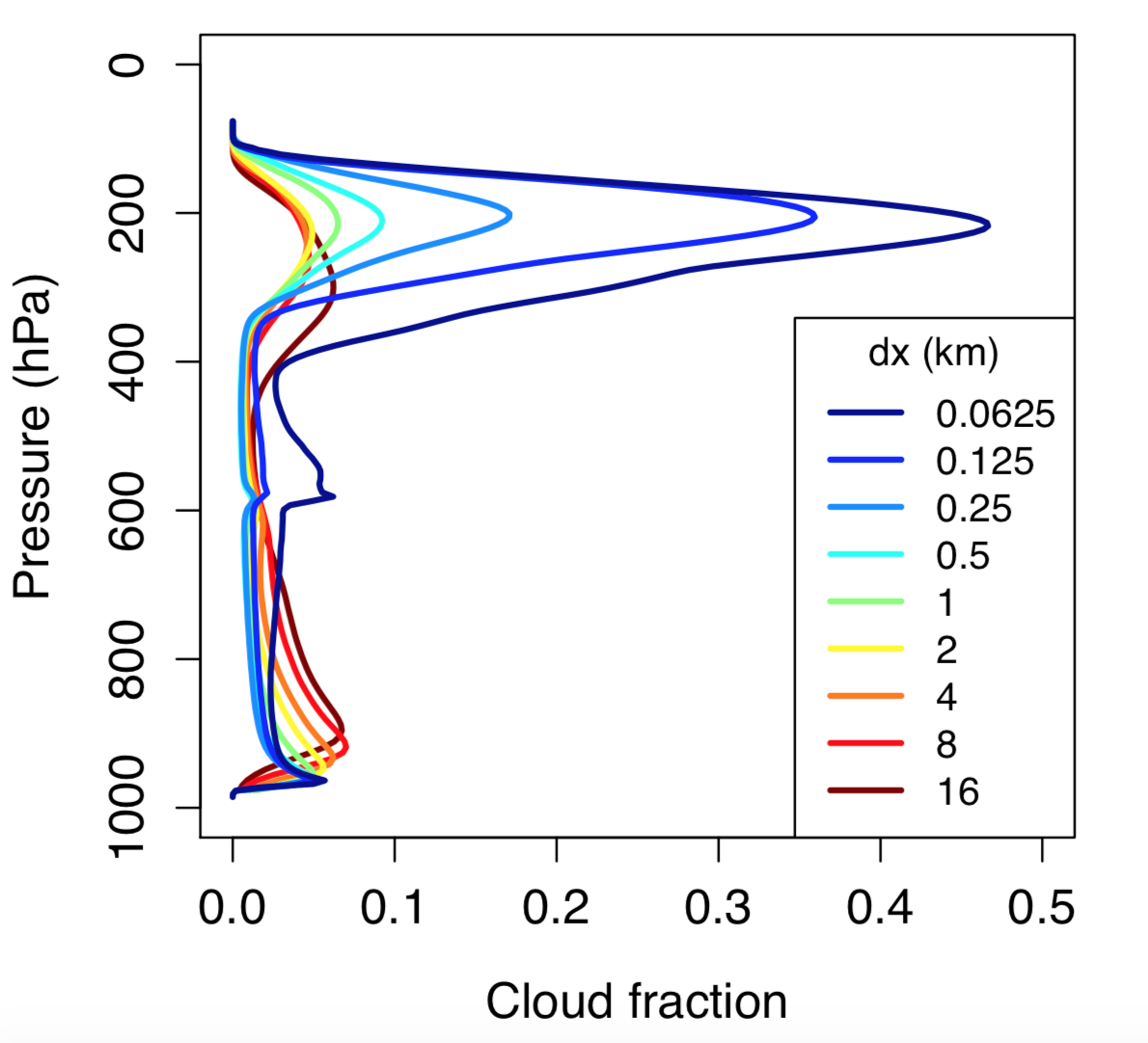
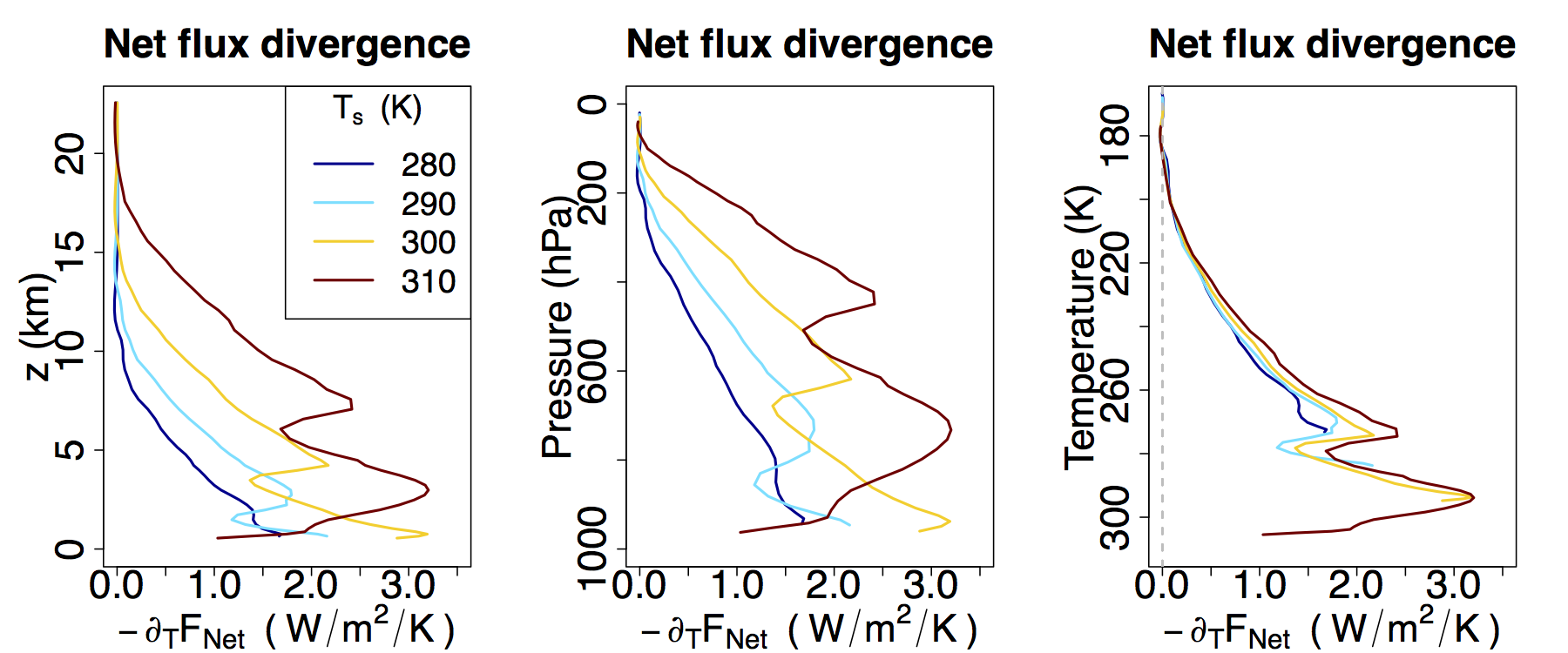
Tropical high clouds ("anvils") mask outgoing infrared radiation and are thus an important player in the climate system. Our ability to simulate them, however, is known to be limited. Here we point out a further limitation, namely that even in cloud-resolving models, anvil cloud area is highly resolution-dependent (figure left). This resolution dependence is understood using the theory of Seeley et al. (2019), through which we demonstrate that at higher resolutions, mixing is more efficient at diluting convective plumes, reducing the efficiency with which they produce precipitation. Thus a greater number of plumes is required to produce the usual average rain rate (~3 mm/day), leading to greater high cloudiness. For details see Jeevanjee and Zhou (2022), as well as follow-up work in Hu et al. (2024).
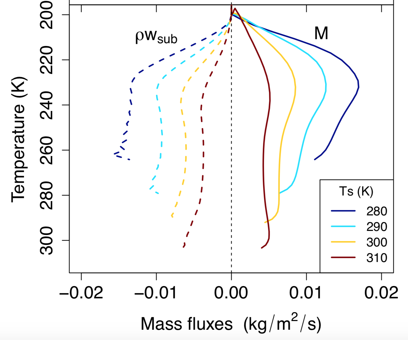
Additional work has explored the dependence of convection on surface temperature, rather than resolution. There exist a few different rules of thumb for how convection should change with warming, but perhaps the most robust is shown at right: convective mass fluxes decrease throughout the troposphere with warming, especially when evaluated in temperature coordinates (i.e. on isotherms). These convective mass fluxes M are constrained to be equal and opposite to the subsidence mass flux ρwsub (dashed lines), which are well understood theoretically. This constraint is found to be more robust than other constraints pertaining to anvil clouds or to convective mass fluxes at cloud-base; for details see Jeevanjee (2022). Follow-up work by Williams and Jeevanjee (2025) further showed that this decrease in mass flux on isotherms is quantitatively constrained to be about 3-4 %/K.
CO2 Radiative Forcing
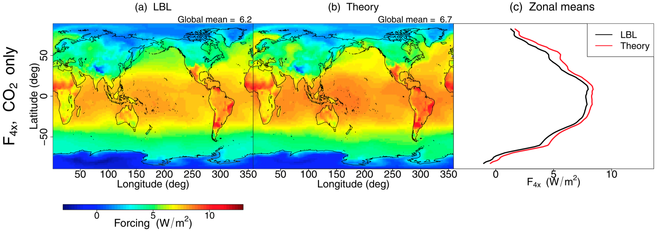
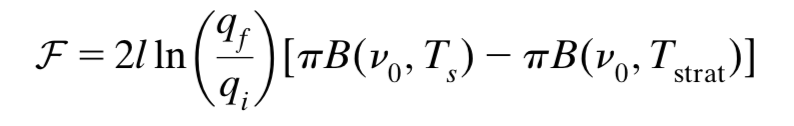
CO2 radiative forcing is a central quantity in climate science and is accurately modeled, but the intricacies of radiative transfer have rendered a chalkboard understanding of this quantity elusive. Building off prior work we construct an analytical model for CO2 forcing which reproduces the results from comprehensive radiative transfer codes with surprising accuracy (figure right), and more importantly provides insight into how CO2 forcing depends on atmospheric state, and thus why it varies so dramatically over the globe. See Jeevanjee et al. (2021) for details,
and this newsletter for a short overview.
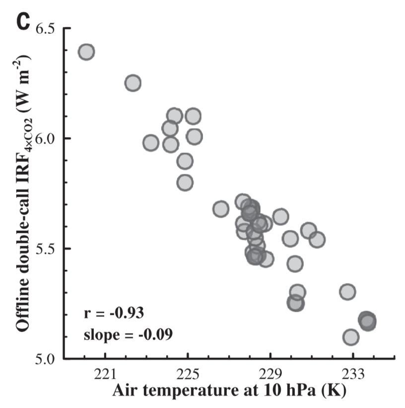
Moreover, the analytical model above suggests that stratospheric temperatures play a key role in determining CO2 forcing. This suggestion was confirmed in follow-up work of He et al. (2021), who found that this state-dependence of CO2 forcing manifests in climate model simulations, and explains much of the variance in CO2 forcing across climate models.
Figure left: Strong correlation between CO2 forcing of various climate models (individual circles), all calculated offline with the same radiation code, and each model's mean stratospheric temperature (evaluated at 10 hPa or a height of 30 km).
Clear-sky Climate Feedbacks
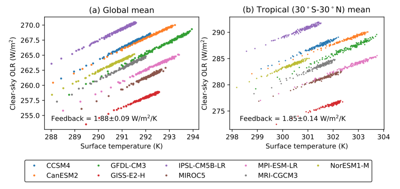
While particular climate feedbacks, such as the water vapor feedback, are known to vary significantly amongst models, the total infrared clear-sky feedback parameter is actually quite robust across models and the model hierarchy, and can be understood with pencil-and-paper. Zhang, Jeevanjee, and Fueglistaler (2020) studied this feedback parameter across GCMs and found a strikingly narrow range of values, clustered around 1.9 W/m2/K (slope of curves in panel a, figure left). They furthermore showed that the `super greenhouse effect', or negative values of this feedback parameter over certain regions in the tropics, cancels out in the tropical average (panel b) due to a robust invariance of global relative humidity distributions under global warming.
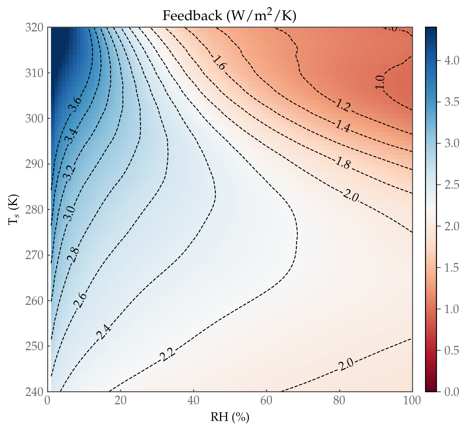
This robustness of the clear-sky feedback parameter in GCMs was put into context by McKim, Jeevanjee, and Vallis (2021), who calculated the clear-sky feedback parameter for idealized tropical atmospheric columns across a range of relative humidity (RH) and surface temperature values (figure right). This figure is dominated by the 2.2 W/m2/K contour, close to the value obtained above in GCMs. At tropical surface temperatures of 290 K and warmer, however, smaller values of the feedback parameter arise, especially at larger RH values. This helps explain the slightly smaller GCM values found above, as well as the non-linearity of feedbacks at high temperatures.
The preferred clear-sky feedback value of roughly 2 W/m2/K can also be understood theoretically, with a simple pencil-and-paper calculation. See Eq. (28) of
Jeevanjee (2018).
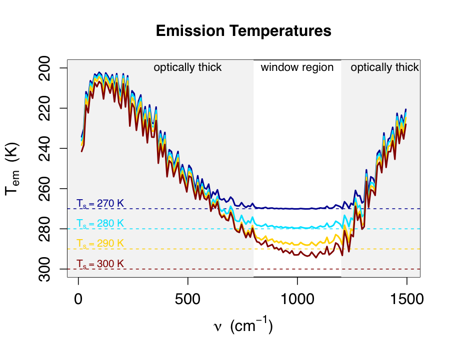
A key ingredient in understanding the 2 W/m2/K clear-sky feedback is "Simpson's Law", which says that for frequencies dominated by the water vapor greenhouse effect, increases in emission to space with warming come largely from the surface, rather than the atmosphere (figure left). This fact has been known for decades but not verified in detail. We provide such a verification here, and also demonstrate the corollary that conventional climate feedbacks must cancel at water-vapor dominated frequencies, explaining the well-known compensation between e.g. the water vapor and lapse rate feedbacks. These results also explain the relative simplicity of the alternative relative-humidity-based feedback, which exhibits no such compensation. For details, see Jeevanjee, Koll, and Lutsko (2021).
A companion paper builds on this progress and develops an analytic model for the longwave clear-sky feedback. The model captures Simpson's Law as well as corrections to it, and also captures the characteristic value of 2 W/m2/K as well as deviations from this value found in the deep tropics. For details, see Koll, Jeevanjee, and Lutsko (2023).
Fundamentals of Radiative Cooling, and Connection to Precipitation Change
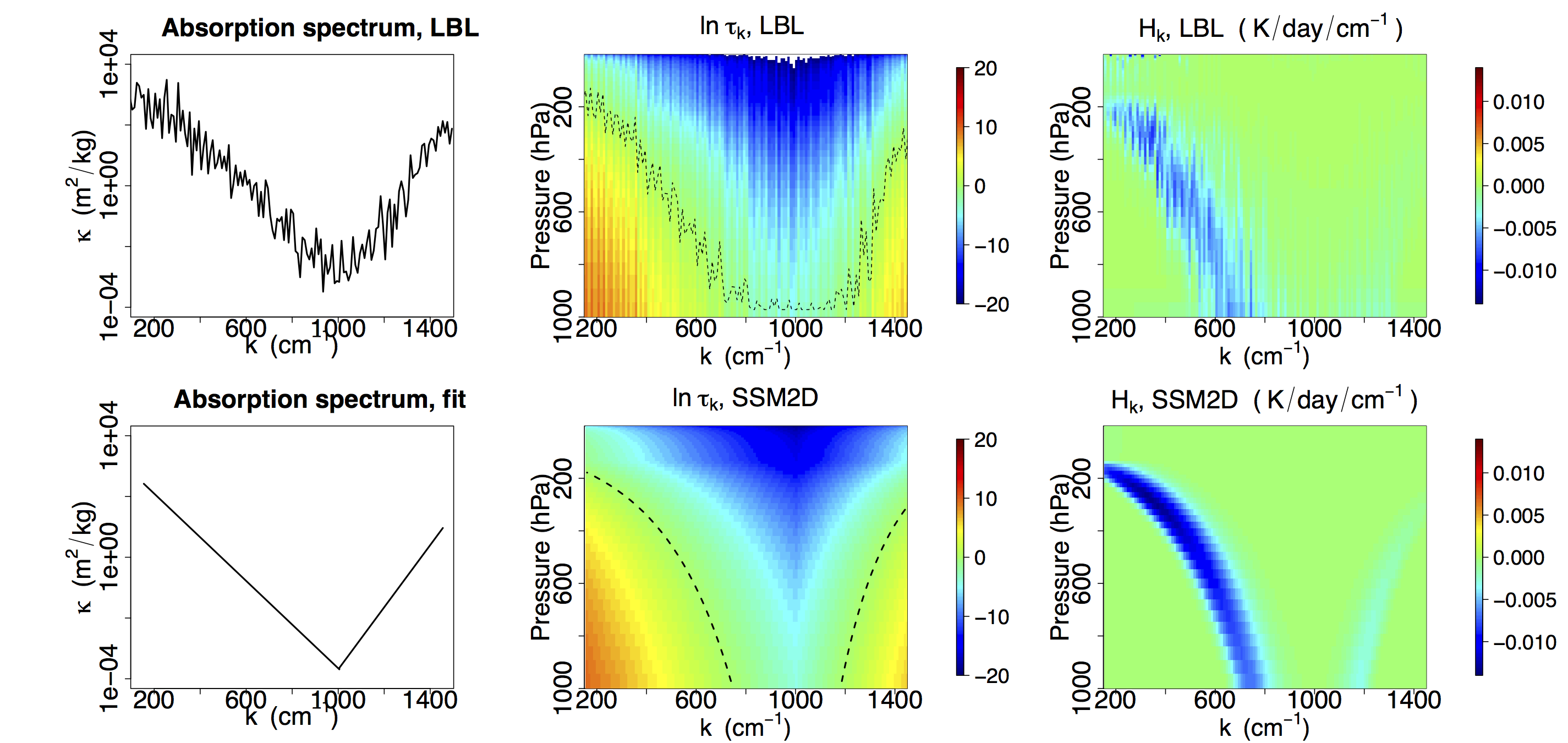
Radiative cooling is tightly linked to weather and atmospheric motions, but remains enigmatic due to the complexity of greenhouse gas spectroscopy and radiative transfer. To address this we develop Simple Spectral Models (SSMs) of radiative cooling (figure right) which emulate our most comprehensive models, but are simple enough to answer basic questions such as why the atmosphere cools at roughly 2 K/day around the globe, or why radiative cooling declines sharply in the upper troposphere at roughly 220 K, only to then rebound in the stratosphere. For details, see Jeevanjee and Fueglistaler (2020a).
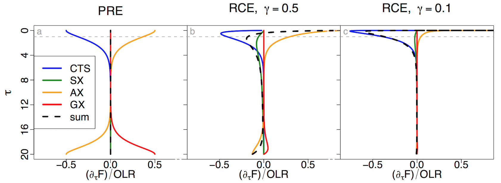
A key ingredient in the SSMs discussed above is the "Cooling-to-Space" (CTS) approximation, which says that radiative cooling of an atmospheric layer is dominated by that layer's cooling-to-space, with exchange between atmospheric layers being negligible. This approximation has been utilized for decades but not fully understood, and is known to break down in some case like Pure Radiative Equilibrium (PRE, figure left, panel a). We study this approximation in detail, and find that a single parameter γ determines its validity, where γ depends on the vertical profiles of temperature as well as greenhouse gas concentration. As γ decreases, the CTS term dominates relative to the exchange terms, and all terms near the surface are suppressed (figure left, panels b and c). For more, see Jeevanjee and Fueglistaler (2020b).
Global mean precipitation is known to roughly balance global mean radiative cooling, and in simulations both increase with surface warming at a rate of roughly 2% per degree C. The origin of this value is not well understood, however. We explain this value by leveraging a novel invariance which radiative cooling profiles exhibit when calculated using temperature as a vertical coordinate (figure right). This invariance leads to a simple picture in which column-integrated radiative cooling is governed primarily by the depth of the troposphere, when measured in temperature coordinates. For more, see Jeevanjee and Romps (2018). (SI can be found here, and an alternate description of this work here).
Entrainment in Idealized Convection
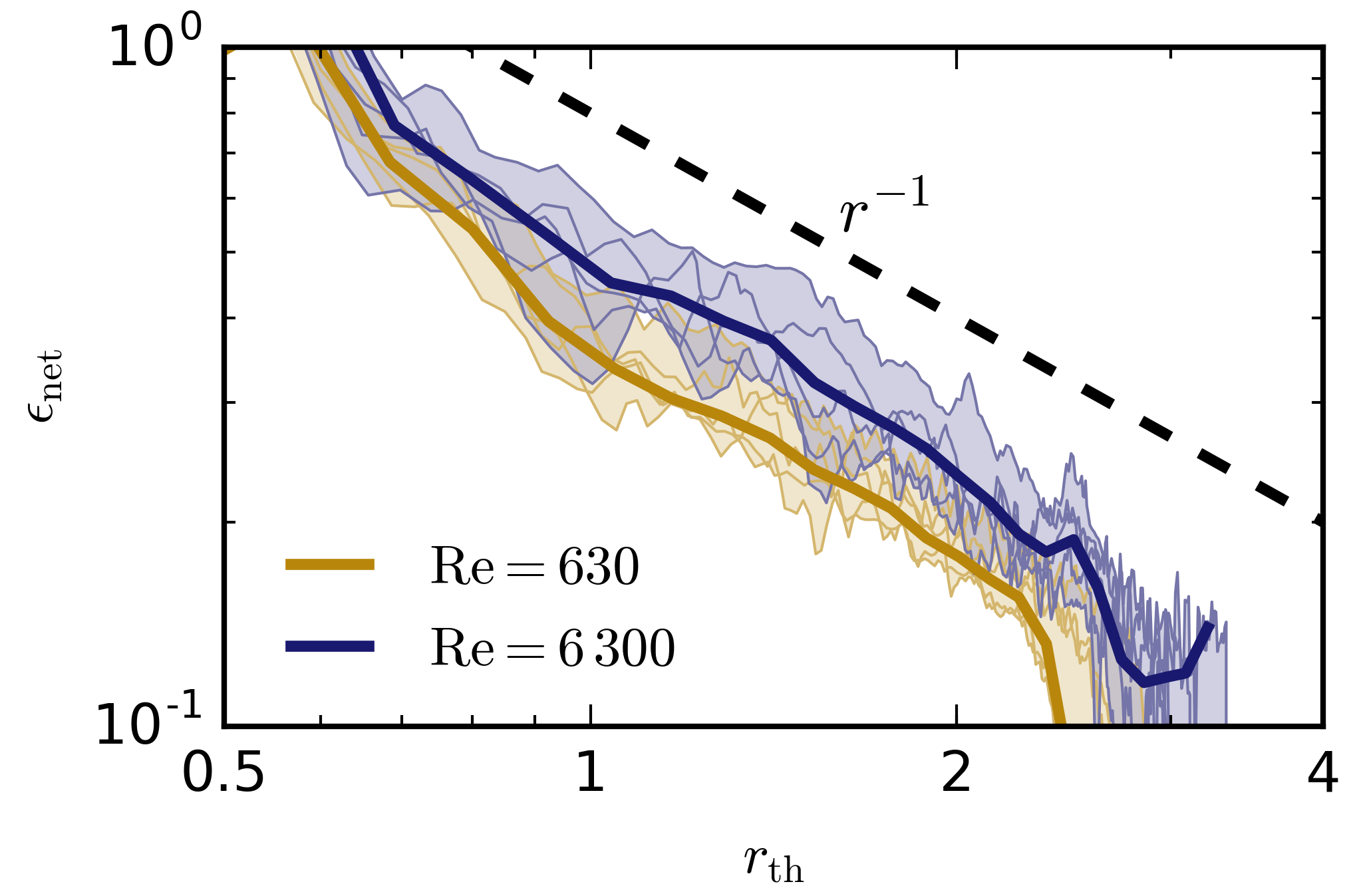
Understanding entrainment, or mixing between a fluid parcel and its environment, has been a long-standing challenge in atmospheric science. In particular, various scaling laws for entrainment have been proposed but not verified, and the relationship of entrainment to turbulence has not been clarified. We approach these issues by studying idealized, dry (i.e. no moisture) buoyant parcels known as thermals, using direct numerical simulation. We find that fractional entrainment indeed obeys a 1/r scaling as previously postulated (r is the thermal's radius), and also find that entrainment is surprisingly insensitive to Reynolds number, i.e. turbulence (figure right). These results are reported in Lecoanet and Jeevanjee (2019), and animations can be found here.
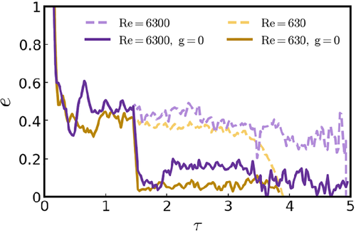
Follow-up work derives an analytical theory for the dynamics of these thermals in which entrainment is driven not by turbulence but by buoyancy, via a set of dynamical constraints. We confirm the central role of buoyancy through mechanism-denial experiments in which gravity is turned off midway through a simulation, where we find that entrainment is drastically reduced without buoyancy (figure left). These results are reported in McKim, Jeevanjee, and Lecoanet (2019).
Another aspect of the dynamics of thermals is the degree to which they experience drag. Although solid objects moving in a fluid typically experience drag, this may not be the case when the object of interest is itself composed of fluid. This question was explored for dry thermals in Morrison, Jeevanjee, and Yano (2022), who indeed found that the drag coefficient Cd for laminar thermals is essentially zero, but slightly negative for turbulent thermals.
Effective Buoyancy
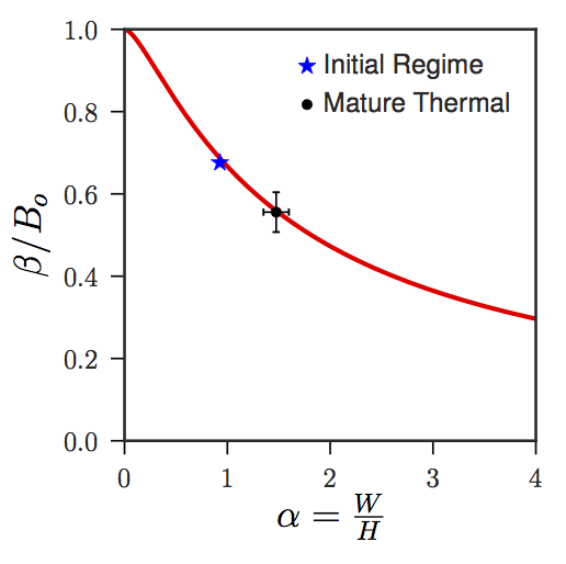
The 'effective buoyancy' of an accelerating parcel is its Archimedean buoyancy B minus an offset, due to the parcel having to push some of the environmental fluid out of its way. This offset grows with parcel aspect ratio, so that wider parcels (at fixed height) accelerate less. Through a novel correspondence with the equations of magnetostatics, we find exact analytical expressions for this offset for idealized parcels with uniform B, and show that these expressions also apply to turbulent, heterogenous parcels (figure left). These expressions describe the `virtual mass' effect for fluid parcels, as well as the compensating subsidence in their environment. See Tarshish et al. (2018) for complete details.
An earlier approach to some of these questions, which emphasizes how this offset of B is enhanced when parcels are near the surface, can be found in Jeevanjee and Romps (2016). An application of these ideas to understanding how simulated convection depends on model grid spacing is given in "Vertical Velocity in the Gray Zone", Jeevanjee (2017), discussed below.
Vertical Velocity in the Gray Zone
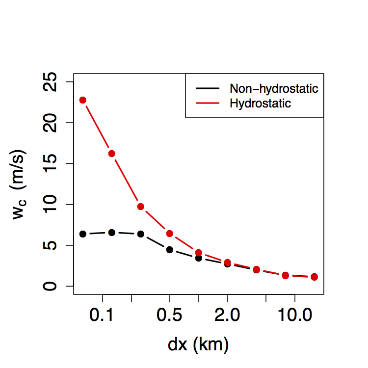
Increasing computer power allows global atmospheric models to be run in a `gray zone' of horizontal resolution which permits but does not fully resolve convection. It is unclear where this gray zone ends, however, and how it is affected by the oft-employed hydrostatic approximation. We address these questions using GFDL's flagship FV3 dynamical core, running simulations across the gray zone both with and without the hydrostatic approximation. We find that horizontal resolutions of approximately 100 m are required for convective vertical velocities wc to converge, and that the hydrostatic approximation over-estimates wc at these resolutions by a factor of 2 - 3 (see figure right). These behaviors of wc can be described by simple analytical formulae, which also map out how wc behaves throughout the gray zone.
See Jeevanjee (2017) for details, and here for an animation of cloud-resolving FV3. During the course of this study we also found a striking dependence of the modeled convection on the explicit damping used to dissipate grid-scale noise. This was investigated further in Anber et al. (2018).
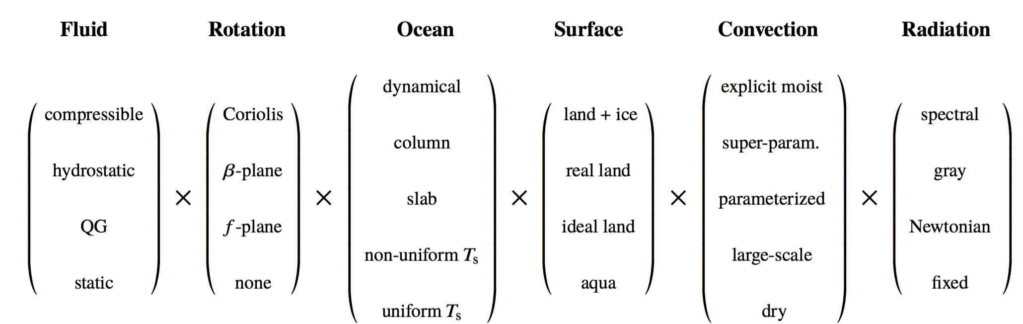
Climate Model Hierarchies
Inspired by the WCRP's recent Model Hierarchies Workshop, we attempted to survey and synthesize some of the current thinking on climate model hierarchies. We give a few formal descriptions of the hierarchy (see figure below), and survey its various uses. We also discuss some of the pitfalls of contemporary climate modeling, and to what extent the `elegance' advocated for by Held (2005) has been used to address them. See Jeevanjee et. al. (2017) for more.
Effective Buoyancy, Inertial Pressure, and Convective Triggering
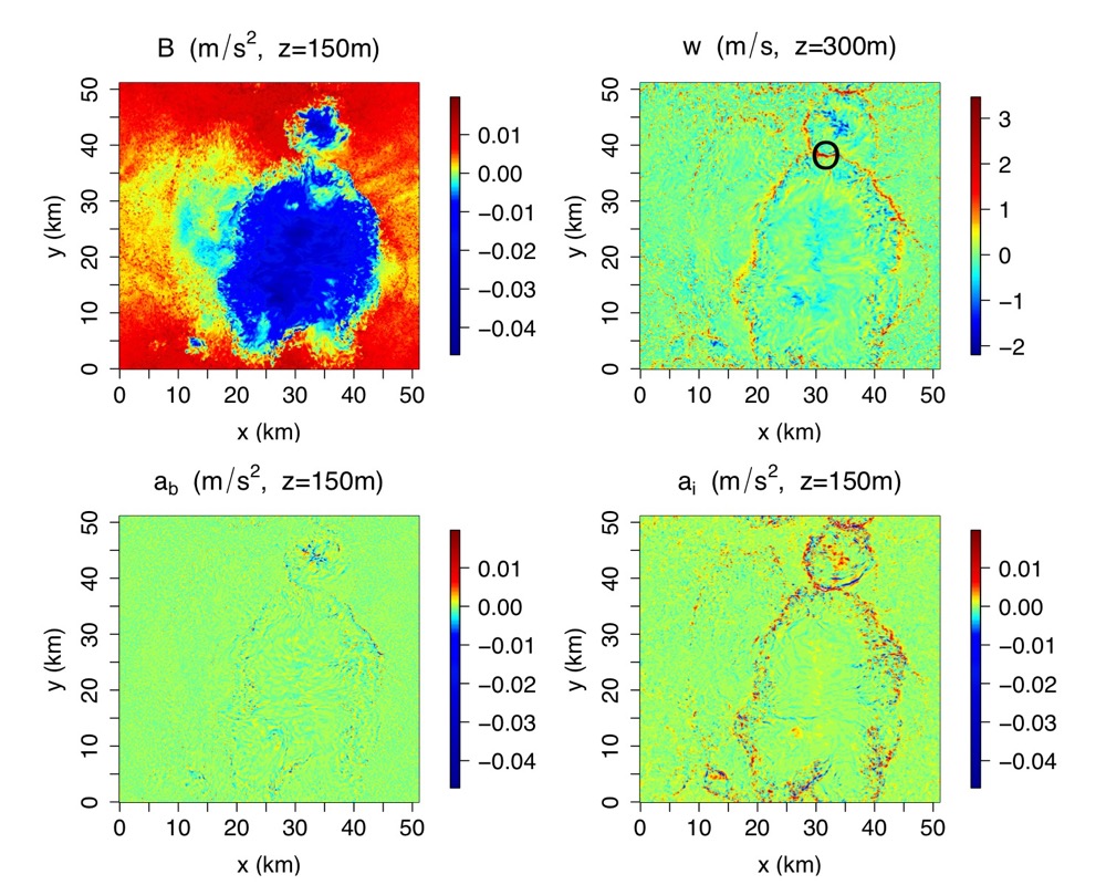
The other force besides effective buoyancy acting on convecting parcels is the inertial (or dynamic) pressure force. In tropical deep convection, most new convection is generated on the edges of 'cold pools' of air produced by evaporation of rain from existing convection. (A large cold pool is visible in the B field in the figure to the right, and the triggered convection along its edge is visible in the w field). It had long been thought that inertial pressure was responsible for this triggering, but the results of Tompkins (2001) suggested that effective buoyancy might also contribute. We helped settle this question by numerically solving the Poisson equations for both effective buoyancy and inertial acceleration in a simulation of tropical convection, showing that indeed the inertial acceleration dominates (bottom row of figure).
See Jeevanjee and Romps (2015) for details.
Convective Self-aggregation
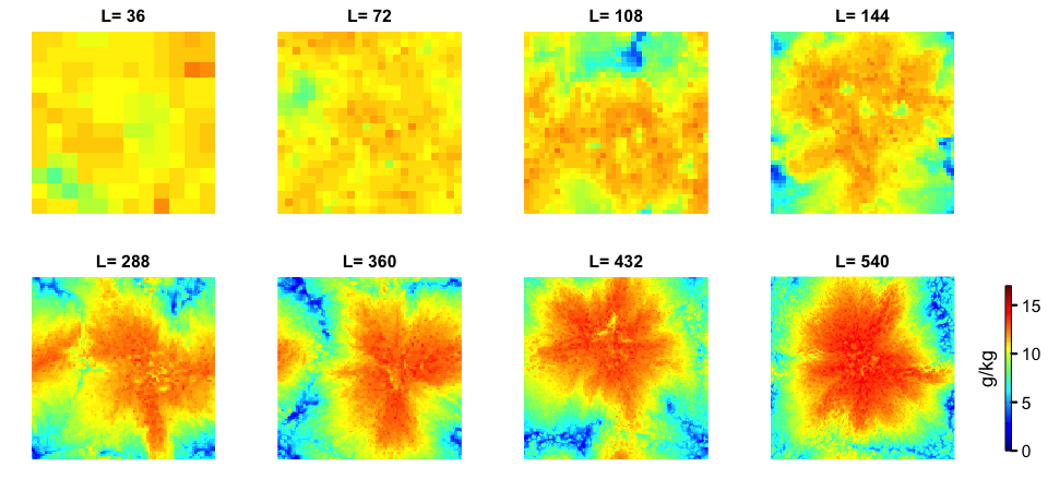
Simulations of tropical convection can spontaneously develop large-scale circulations even in the absence of any large-scale forcing, in a phenomenon known as "self-aggregation". This large-scale circulation partitions the atmosphere into moist and dry regions, as can be seen in the individual panels to the left. Such self-aggregation had previously only been seen in simulations with a domain larger than ~ 300 km on a side, but by disabling cold pools in our simulation, we obtained aggregation at all domain sizes (see figure).
See Jeevanjee and Romps (2013) for details.